Introduction

ColiCoords is a python project aimed to make analysis of fluorescence microscopy data from rodlike cells more streamlined and intuitive. These goals are achieved by describing the shape of the cell by a 2nd degree polynomial, and this simple mathematical description together with a data structure to organize cell data on a single cell basis allows for straightforward and detailed analysis.

Using ColiCoords

The basic princlples of ColiCoords will first be demonstrated with a simple example. We start out with a binary, brightfield and fluorescence image of a horizontally oriented cell. To turn this data into a Cell object we need to first create a Data class and use the add_data() method to add the images as an ndarray, as well as indicate the data class (binary, brightfield, fluorescence or storm). This data interally within the Cell object as well as to initialize it.

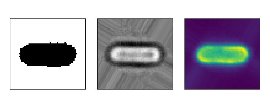
Binary (left), brightfield (middle) and fluorescence (right) input images.

import tifffile
from colicoords import Data, Cell

binary_img = tifffile.imread('data/01_binary.tif')
brightfield_img = tifffile.imread('data/01_brightfield.tif')
fluorescence_img = tifffile.imread('data/01_fluorescence.tif')

data = Data()
data.add_data(binary_img, 'binary')
data.add_data(brightfield_img, 'brightfield')
data.add_data(fluorescence_img, 'fluorescence', name='flu_514')

cell = Cell(data)

The Cell object has two main attributes: data and coords. The data_dict attribute is the instance of Data used to initialize the Cell object and holds all images as ndarray subclasses in the attribute data_dict. The coords attribute is an instance of Coordinates and is used to optimize the cell’s coordinate system and perform related calculations. The coordinate system described by a polynomial of second degree and together with left and right bounds and the radius of the cell they parameterize the coordinate system. These values are first initial guesses based on the binary image but can be optimized iteratively:

cell.optimize()

More details on optimization of the coordinate system can be found in the section Coordinate Optimization. The cells coordinate system allows for the conversion of carthesian input coordinates to be transformed to cell coordinates. The details of the coordinate system and applications are described in section Coordinate System.

Plotting radial distributions

In this section we will go over an example of plotting the radial distribution of the input fluorescence image. ColiCoords can plot distribution of signals from both image or localization-based (see also Processing of SMLM data) data along both the longitudinal or radial axis.

from colicoords.plot import CellPlot
import matplotlib.pyplot as plt

cp = CellPlot(cell)

plt.figure()
cp.imshow('flu_514', cmap='viridis', interpolation='nearest')
cp.plot_outline()
cp.plot_midline()
plt.show()

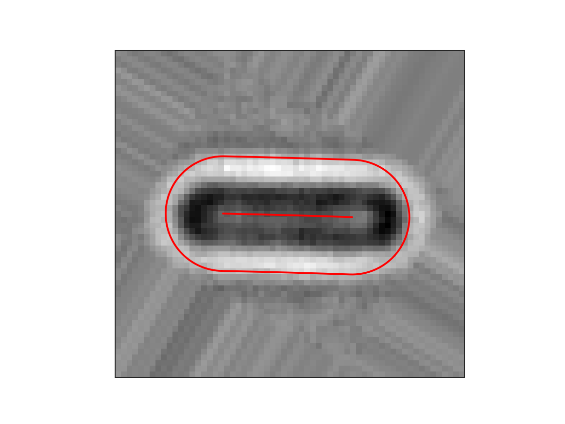
Brightfield image with cell midline and outline.

This shows the brightfield image together with the cell outline and midline optimized from the binary image, which was derived from the brightfield image. As can be seen the coordinate system does not completely match the fluorescence image of the cell. This is because the binary image is only a crude estimation of the actual cell position and shape. The coordinate system can be optimize based on the brightfield image to refine the coordinate system. Other input data channels (fluorescence, storm) can be used as described in the section Coordinate Optimization.

cell.optimize('brightfield')
cell.measure_r('brightfield', mode='min')

Here, the first line optimizes the coordinate system to match the shape of the cell as its measured in the brightfield image through an iterative bootstrapping process. Then, in the second line, the radius of the cell is determined from the brightfield image. The keyword argument mode=’min’ indicates that in this case the radius of the cell is defined as where the pixel values on the radial distribution are minimum. Note that this value for the radius is not used in transforming coordinates from carthesian to cell coordinates but only in geometrical properties such as cell area or volume. This gives the following result:

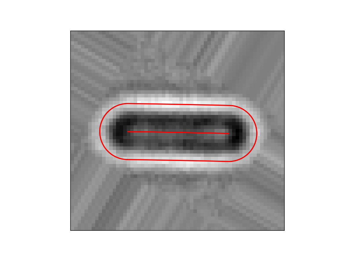
Brightfield image with optimized coordinate system.

To plot the radial distribution of the flu_514 fluorescence channel:

f, (ax1, ax2) = plt.subplots(1, 2)
cp.plot_r_dist(ax=ax1)
cp.plot_r_dist(ax=ax2, norm_x=True, norm_y=True)
plt.tight_layout()

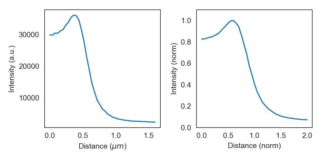
Radial distribution curve of fluorescence as measured (left) and normalized (right).

The displayed curve is constructed by calcuating the radial distance for every the (x, y) coordinates pair for each pixels. The final curve is calculated from all datapoints by convolution with a gaussian kernel.

The data can be accessed directly from the Cell object by calling r_dist. The radial distribution curves can be normalized in both x and y directions. When normalized in the x direction the radius obtained from the brightfield image is set to one, thereby eliminating cell-to-cell variations in width.