Batch Processing
ColiCoords provides utility functions to easily convert stacks of images of cells optionally together with
single-particle localization data (STORM). Binary images of the cells are required to identify the cells positions as
well as to determine their orientation to horizontally align the cells. All preprocessing on input data such as background
correction, flattening, alignment or drift correction needs to be done before the data is input into ColiCoords.
The segmentation process to generate binary images does not need to be done with high accuracy since the binary is only used to identify the position and calcuate initial guesses for the coordinate system. Optimization of the coordinate system can be done in a second step based on other input images (e.g. brightfield or STORM/PAINT membrane marker).
The segmentation can be done via classical methods such as thresholding and watershedding or though cell-analysis software such as CellProfiler or Ilastik. In the CNN module of ColiCoords provides the user with a Keras/Tensorflow implementation the the U-Net convolutional neural network architecture [1505.04597]. The networks are fast an robost and allow for high-troughput segmentation (>10 images/second) on consumer level graphics cards. Example notebooks can be found in the examples directory with implementations of training and applying these neural networks.
Making a Data object
After preprocessing and segmentation, the data can be input into ColiCoords. This is again handled by the
Data object. Images are added as ndarray whose shape should be identical.
STORM data is input as Structured Arrays (see also Processing of SMLM data).
A Data object can be prepares as follows:
import tifffile
from colicoords import Data, data_to_cells

binary_stack = tifffile.imread('data/02/binary_stack.tif')
flu_stack = tifffile.imread('data/02/brightfield_stack.tif')
brightfield_stack = tifffile.imread('data/02/fluorescence_stack.tif')

data = Data()
data.add_data(binary_stack, 'binary')
data.add_data(flu_stack, 'fluorescence')
data.add_data(brightfield_stack, 'brightfield')
The Data class supports iteration and Numpy-like indexing. This indexing capability is
used by the helper function data_to_cells() to cut individual cells out of the data
across all data channels. Every cell is then oriented horizontally based on the image moments in the binary image (as default).
A name attribute is assigned based on the image the cell originates from and the label in the binary image, ie
A Cell object is initialized together with its own coordinate system and placed in an instance of
CellList. This object is a container for Cell objects and supports
Numpy-like indexing and allows for batch operations to be done on all cells in the container.
To generate Cell objects from the data and to subsequently optimize all cells’ coordinate
systems:
Cell objects and optimization
cell_list = data_to_cells(data)
cell_list.optimize('brightfield')
cell_list.measure_r('brightfield', mode='mid')
High-performance computing is supported for timely optimizing many cell object though calling optimize_mp() (see Coordinate Optimization).
The returned CellList object is basically an ndarray of colicoords.cell.Cell objects. Many of the single-cell attributes can be accessed which are returned in the form of a list or array for the whole set of cells.
Plotting
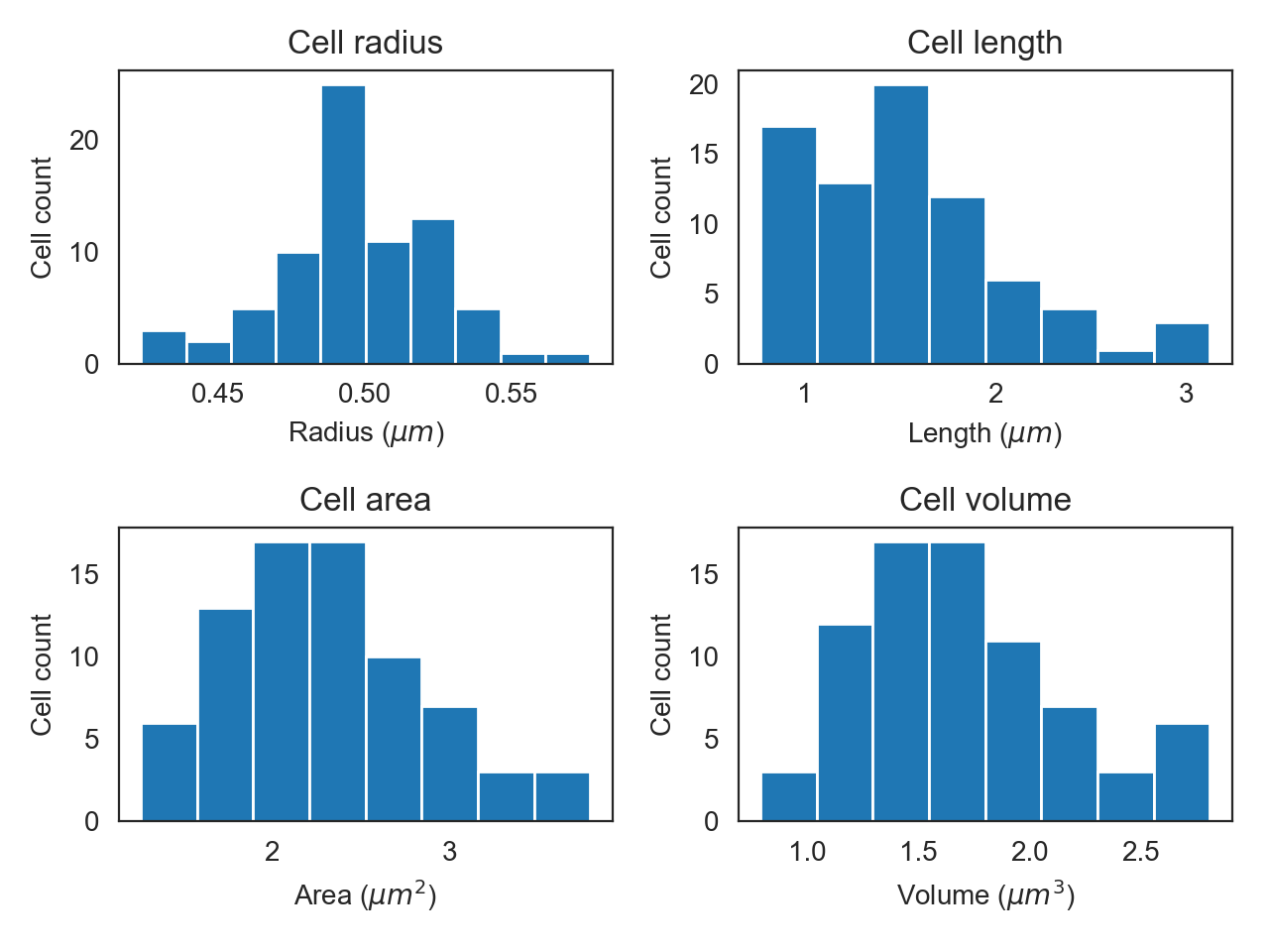
CellListPlot can be used to easily plot fluorescence distribution of the set of cells or histogram certain properties.
from colicoords import CellListPlot

clp = CellListPlot(cell_list)
fig, axes = plt.subplots(2, 2)
clp.hist_property(ax=axes[0,0], tgt='radius')
clp.hist_property(ax=axes[0,1], tgt='length')
clp.hist_property(ax=axes[1,0], tgt='area')
clp.hist_property(ax=axes[1,1], tgt='volume')
plt.tight_layout()
When using CellList the function r_dist() returns the radial distributions of all cells in the list.
x, y = cell_list.r_dist(20, 1)
Here, the arguments given are the stop and step parameters for the x-axis, respectively. The returned y is an array where each row holds the radial distribution for a given cell.
To plot the radial distributions via CellListPlot:
f, axes = plt.subplots(1, 2)
clp.plot_r_dist(ax=axes[0])
axes[0].set_ylim(0, 35000)
clp.plot_r_dist(ax=axes[1], norm_y=True, norm_x=True)
plt.tight_layout()
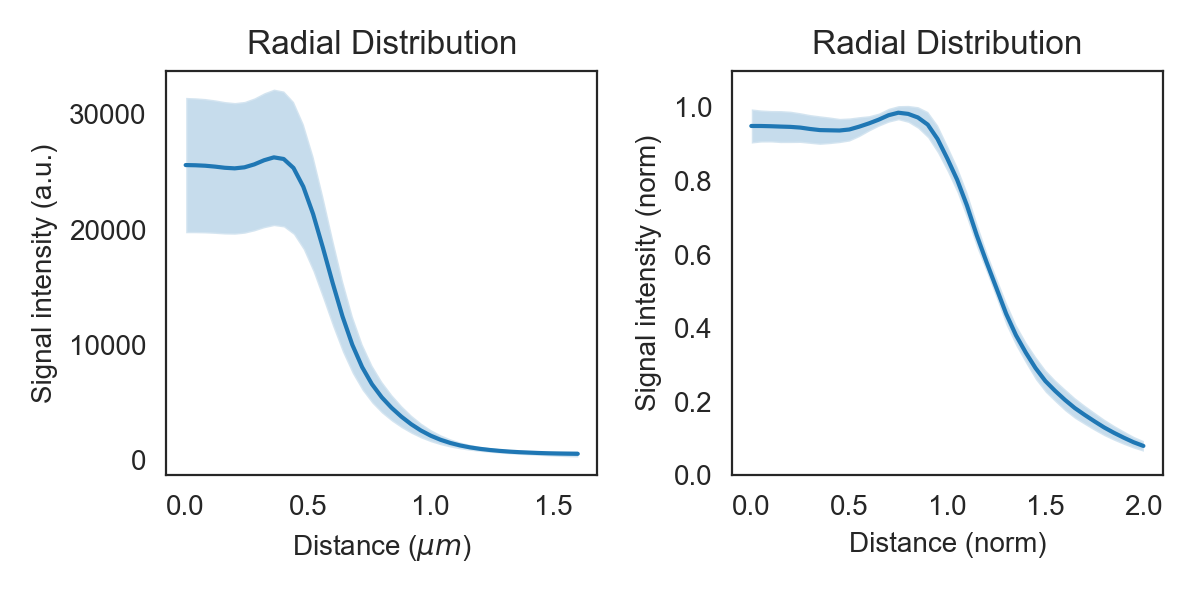
The band around the line shows the sample’s standard deviation. By normalizing each curve on the y-axis variation in absolute intensity is eliminated and the curve shows only the shape and its standard deviation. Normalization on the x-axis sets the radius measured by the brightfield in the previous step to one, thereby eleminating cell width variations.
| [RFB15] | Olaf Ronneberger, Philipp Fischer, and Thomas Brox. U-net: convolutional networks for biomedical image segmentation. 2015. arXiv:arXiv:1505.04597. |